How to Use the Interpolation Calculator
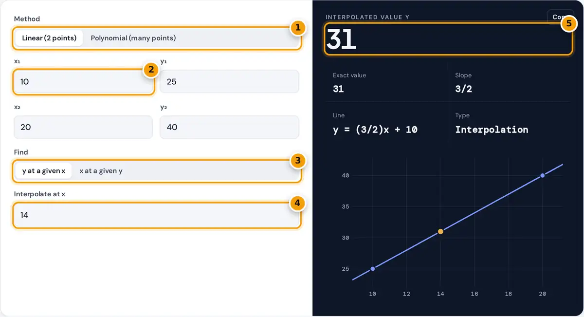
- Choose linear interpolation for two points or polynomial interpolation for many.
- Enter the known points, x₁ and y₁ then x₂ and y₂.
- Find y at a given x, or switch to find x at a given y.
- Enter the x value to interpolate at.
- Read the estimate, the line equation and whether it is interpolation or extrapolation.
For Linear interpolation, enter two known points (x₁, y₁) and (x₂, y₂) and the x value you want to estimate. Choose x at a given y to run the calculation backwards, for example to find the time at which a reading reached a target. For Polynomial interpolation, paste your data with one x, y pair per line, up to 12 points, and enter the x value to evaluate.
The result panel shows the estimate as an exact fraction and a decimal, the slope or degree, the equation of the fit and whether the point lies inside the data range (interpolation) or outside it (extrapolation). The graph plots the data, the fitted line or curve, and the estimated point. Below the tool, the formula is written out with your numbers, and in polynomial mode the full divided difference table is shown.
Linear Interpolation Formula
Solved for x: x = x₁ + (y − y₁) × (x₂ − x₁) ÷ (y₂ − y₁)
The formula assumes the quantity changes at a constant rate between the two points, so the estimate lies on the straight line joining them. The fraction (x − x₁) ÷ (x₂ − x₁) says how far along the interval you are, and the same fraction of the change in y is added to y₁.
Worked Examples
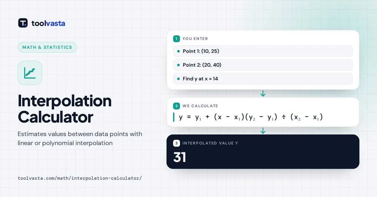
Linear: a table gives 25 at x = 10 and 40 at x = 20. Estimate the value at x = 14. The slope is (40 − 25) ÷ (20 − 10) = 1.5, so y = 25 + (14 − 10) × 1.5 = 25 + 6 = 31. The point is 40% of the way along the interval.
Polynomial: the points (0, 1), (1, 3), (2, 11) and (3, 31) have divided differences 2, 8, 20 in the first column, 3, 6 in the second and 1 in the third. The Newton form is P(x) = 1 + 2x + 3x(x − 1) + x(x − 1)(x − 2), which expands to x³ + x + 1. At x = 1.5, P(1.5) = 3.375 + 1.5 + 1 = 5.875 = 47/8. Straight-line interpolation between (1, 3) and (2, 11) would give 7, so the curvature matters here.
Lagrange and Newton Polynomials
Through n points with different x values there is exactly one polynomial of degree at most n − 1. The Lagrange form builds it from basis polynomials that equal 1 at one data point and 0 at all the others:
Newton: P(x) = f[x₀] + f[x₀,x₁](x − x₀) + f[x₀,x₁,x₂](x − x₀)(x − x₁) + …
Both forms give the same polynomial. The Newton form is easier to extend, because adding a point only adds one new term, and its coefficients come straight from the top row of the divided difference table.
| Method | Points | Best for |
|---|---|---|
| Linear | 2 | Tables of values, quick estimates, evenly changing data |
| Quadratic | 3 | Data with gentle curvature |
| Cubic and higher | 4 or more | Smooth functions sampled at a few points |
Interpolating in Tables of Values
Printed tables in science, engineering and finance list values only at round numbers, so interpolation fills the gaps. Suppose a table gives 1.002 at 20 and 0.798 at 30, and you need the value at 26. The point is 60% of the way along, so y = 1.002 + 0.6 × (0.798 − 1.002) = 1.002 − 0.1224 = 0.8796. Check the answer by making sure it lies between the two table values.
Tips and Limits
- Interpolation is most reliable inside the data range. Extrapolation beyond the first or last point assumes the trend continues, and polynomial extrapolation in particular can swing far off.
- Using many points does not always help. High-degree polynomials can oscillate between widely spaced points, which is known as Runge's phenomenon. Piecewise linear or low-degree fits are often safer for measured data.
- Every x value must be different. If your data has repeated x values, average them first.
- All arithmetic is exact, so decimals you type are treated as exact fractions.
Frequently asked questions
What is linear interpolation?
It estimates a value between two known points by assuming a straight line joins them. The formula is y = y₁ + (x − x₁)(y₂ − y₁) ÷ (x₂ − x₁).
How do I interpolate between two values in a table?
Take the two rows on either side of your x value. Work out how far along the interval x is, as a fraction, and add that fraction of the change in y to the first y value.
What is the difference between interpolation and extrapolation?
Interpolation estimates a value inside the range of the known data. Extrapolation estimates outside it, which relies on the trend continuing and is usually less accurate.
What is Lagrange interpolation?
A way to build the single polynomial that passes through all your points. Each data point gets a basis polynomial that is 1 at that point and 0 at the others, weighted by its y value.
How many points do I need for polynomial interpolation?
Two points give a line, three give a quadratic and four give a cubic. In general, n points with different x values define one polynomial of degree at most n − 1.
Can I find x for a known y?
Yes. In linear mode choose x at a given y. The same straight line is solved for x, which is useful for finding when a reading reached a target value.