How to Use the Linear Regression Calculator
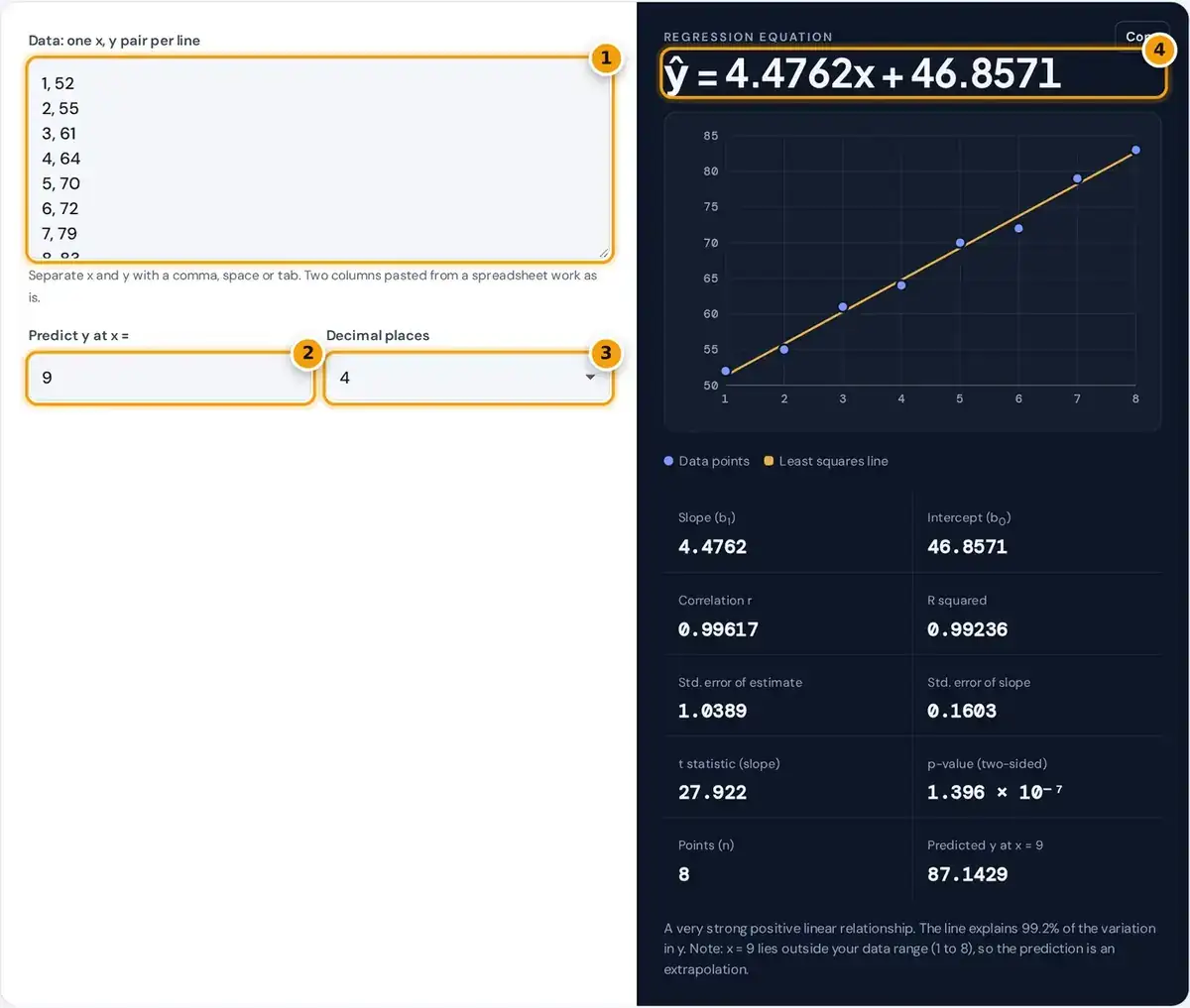
- Paste your data, one x, y pair per line. Two columns copied from a spreadsheet work.
- Enter an x value to predict y for it.
- Choose how many decimal places to show.
- Read the regression equation, then slope, R², p-value and the scatter plot.
Enter your data with one observation per line: the x value, or predictor, first, then the y value, or response. Separate them with a comma, space or tab, with exactly one pair on each line.
You can paste two columns straight from a spreadsheet such as Excel or Google Sheets. The linear regression calculator fits the line and redraws the scatter plot with all your data points as you type.
Enter any x in the Predict box to get its fitted value, and choose the decimal places. The Copy button saves the regression equation with r, R squared, standard error and n for your report.
Least Squares Regression Formulas
Simple linear regression fits a straight line that predicts the dependent variable y from one independent variable x. Ordinary least squares simply picks the line that minimizes the sum of squared residuals, the vertical distances.
The slope is the sum of cross products of deviations from each mean, divided by the sum of squared x deviations. The intercept then places the line through the point formed by the two means.
The NIST/SEMATECH e-Handbook of Statistical Methods describes this as the most widely used modeling method, efficient with small datasets but sensitive to outliers. The regression equation reads: fitted y equals slope times x plus intercept.
Slope b1 = Sxy ÷ Sxx Intercept b0 = ȳ − b1x̄
r = Sxy ÷ √(SxxSyy) R² = r²
Standard error s = √(SSE ÷ (n − 2)) SE(b1) = s ÷ √Sxx
t = b1 ÷ SE(b1), with n − 2 degrees of freedom
Worked Example With Study Hours
This worked example uses the default data: hours of study as x and test score as y for 8 students. The mean of x is 4.5 hours, and the mean test score is 67 points.
From the eight data pairs, Sxx is 42 and Sxy is 188, so the slope is 188 divided by 42, or 4.4762. The intercept is then 67 minus 4.4762 times 4.5, which gives 46.8571 points.
Each extra hour of study is associated with about 4.5 more points on average. The correlation is r = 0.99617, R squared is 0.99236, and the predicted score after 9 hours of study is 87.1429 points.
How to Read the Regression Output
The correlation coefficient r shows the direction and strength of the linear relationship on a scale from minus 1 to 1. R squared, which is r times itself, gives the share of the variation explained.
The standard error of the estimate is the typical size of a residual, in the units of y. In the example it is 1.0389, so a typical score sits about a point from the line.
The t statistic is the slope divided by its standard error, compared with a t distribution with n minus 2 degrees of freedom. The calculator reports a two-sided p-value testing whether the slope is zero.
| Output | What it tells you |
|---|---|
| Slope | Change in y for each one-unit increase in x |
| Intercept | Fitted y when x = 0 (may be meaningless if 0 is far from your data) |
| r | Strength and direction of the linear relationship, from −1 to 1 |
| R squared | Share of the variation in y explained by the line |
| Std. error of estimate | Typical size of a residual, in the units of y |
| p-value | Chance of a slope this far from 0 if there were truly no linear relationship |
Assumptions Behind the P-Value
The slope and intercept are always the best-fitting line in the least squares sense. The standard errors and the p-value, however, rely on extra assumptions about the data and the residuals left over after fitting.
There should be a roughly linear relationship, residuals should be independent with equal spread across the range of x, and should be roughly normally distributed. The Penn State simple linear regression lesson explains each condition.
Always check the scatter plot. A curved pattern means a straight line is the wrong model, and a fan shape, where points spread wider as x grows, means the p-value and standard errors may mislead.
Limits and Good Practice
Correlation is not causation. A strong fit shows that x and y move together, but it cannot prove that x causes y, because a third factor or pure coincidence can produce the same straight-line pattern.
Avoid extrapolation. Predictions outside the range of your x values are flagged, because the relationship may change there. Outliers matter too: one extreme point can move the line, so try removing it to test sensitivity.
This tool fits only one predictor. Multiple regression with several x variables, or logistic regression for yes/no outcomes, needs statistical software. For homework steps with a residual table, see the line of best fit calculator.
- Correlation is not causation.
- Predictions outside your x range are flagged.
- One extreme point can move the line a lot.
- Only one predictor is supported.
Frequently asked questions
What does a linear regression calculator do?
It fits the straight line that best predicts y from x by minimizing the sum of squared residuals. It reports the slope, intercept, correlation, R squared, standard errors and a p-value for the slope.
What is a good R squared value?
It depends on the field. In controlled physics experiments values above 0.99 are common, while in social science 0.3 can be useful. R squared shows how much variation the line explains, not whether the model is right.
What is the difference between r and R squared?
r is the correlation coefficient and shows direction and strength from minus 1 to 1. R squared is r multiplied by itself and gives the share of variation explained, from 0 to 1.
How is the p-value for the slope calculated?
The slope is divided by its standard error to give a t statistic, which is compared with a t distribution with n minus 2 degrees of freedom. The calculator reports the two-sided p-value.
How many data points do I need?
At least 3, because the standard error uses n minus 2 degrees of freedom. More points give more reliable estimates, and a spread of x values across the range you care about helps most.
What does a negative slope mean?
A negative slope means y tends to fall as x rises. The size of the slope tells you how many units y changes, on average, for each one-unit increase in x.