How to Use the Exponential Growth Calculator
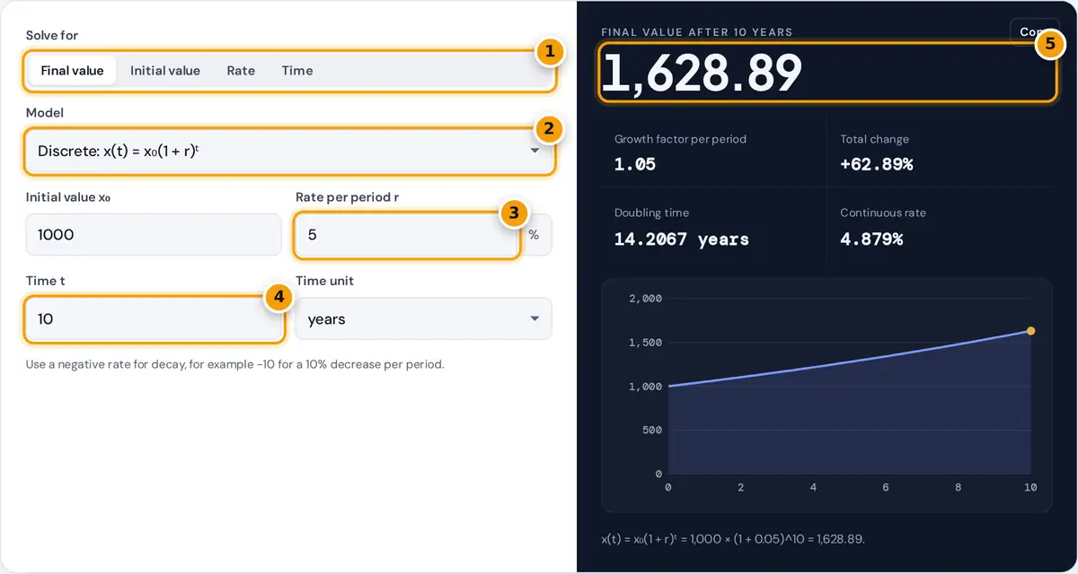
- Choose what to solve for: final value, initial value, rate or time.
- Pick the discrete (1 + r)^t model or continuous e^(rt) growth.
- Enter the rate per period. Use a negative rate for decay.
- Enter the number of periods and choose the time unit.
- Read the answer, the doubling time and the chart of value over time.
Choose what you want to find: the final value, the initial value, the growth rate or the time. Then pick a model. The discrete model, x₀(1 + r)ᵗ, fits growth that happens once per period, such as a population counted every year or interest added once a year. The continuous model, x₀eʳᵗ, fits processes that change smoothly all the time, such as radioactive decay or bacteria in ideal conditions.
Enter the known values. The rate is a percentage per period, and a negative rate gives exponential decay. The time unit is only a label, so make sure the rate and time use the same period. The result panel shows the answer, the growth factor, the total change, the doubling time or half-life and the equivalent rate in the other model, with a chart and a value table.
Exponential Growth Formulas
Rate: r = (x ÷ x₀)¹∕ᵗ − 1 or r = ln(x ÷ x₀) ÷ t
Time: t = ln(x ÷ x₀) ÷ ln(1 + r) or t = ln(x ÷ x₀) ÷ r
Doubling time = ln 2 ÷ ln(1 + r) or ln 2 ÷ r
Here x₀ is the starting amount, r is the rate per period as a decimal (5% = 0.05), t is the number of periods and e ≈ 2.71828. The two models are linked: a discrete rate r equals a continuous rate of ln(1 + r).
Worked Examples
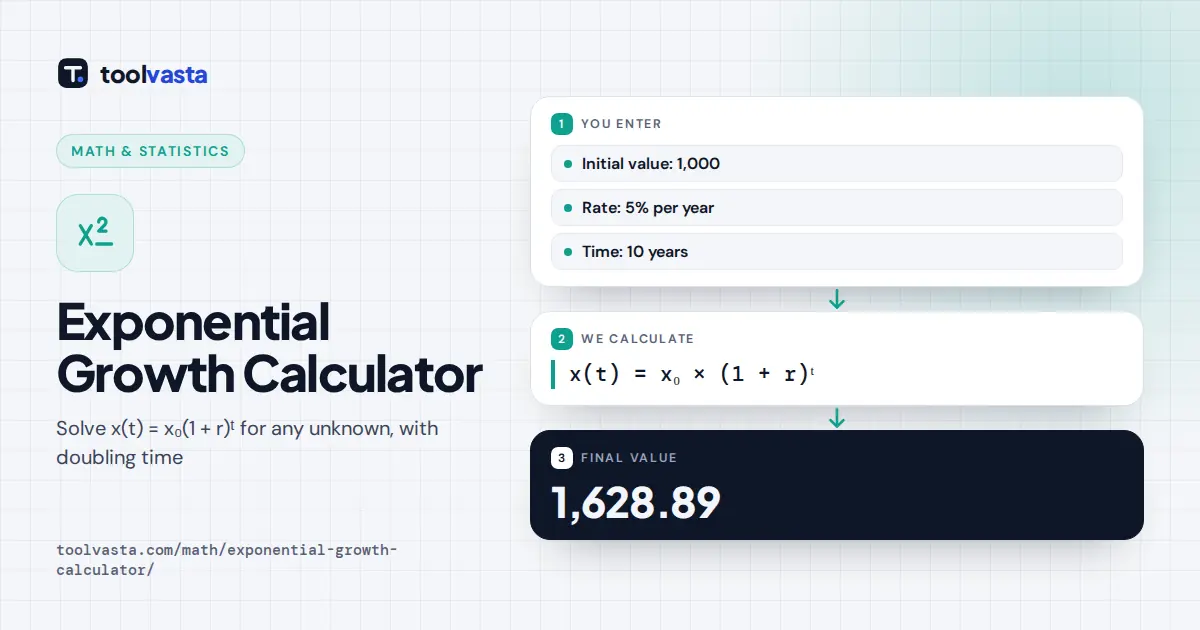
- Final value: 1,000 growing 5% per year for 10 years gives 1,000 × 1.05¹⁰ = 1,628.89. The doubling time is ln 2 ÷ ln 1.05 = 14.2067 years.
- Continuous: the same numbers with eʳᵗ give 1,000 × e⁰·⁵ = 1,648.72, slightly more because growth compounds every instant.
- Rate: a value that doubles from 1,000 to 2,000 in 8 years grows at (2)¹∕⁸ − 1 = 9.0508% per year.
- Time: to triple at 7% per year takes ln 3 ÷ ln 1.07 = 16.2376 years.
- Decay: 500 mg decaying continuously at −10% per hour leaves 500 × e⁻⁰·⁵ = 303.265 mg after 5 hours. The half-life is ln 2 ÷ 0.1 = 6.93147 hours.
Doubling Times at Common Rates
| Rate per period | Exact doubling time (discrete) | Rule of 72 estimate |
|---|---|---|
| 2% | 35.00 | 36 |
| 3% | 23.45 | 24 |
| 5% | 14.21 | 14.4 |
| 7% | 10.24 | 10.3 |
| 10% | 7.27 | 7.2 |
The rule of 72 divides 72 by the percentage rate. It is a quick mental estimate that works best for rates between about 5% and 10%.
Exponential vs Linear Growth
Linear growth adds the same amount each period, while exponential growth multiplies by the same factor. At first the two look similar, but exponential growth soon pulls far ahead because each period’s increase is calculated on a larger base. That is why the chart curves upward for growth and flattens toward zero for decay.
Checking Your Answer
A quick way to check an exponential growth answer is to look at the growth factor and the number of periods. If a quantity grows 5% a year, it is multiplied by 1.05 each year, so after 10 years it must be 1.05 multiplied by itself 10 times, which is about 1.629. Any answer near 1,500 for x₀ = 1,000 would therefore be wrong, because that would be simple (linear) growth of 50 per year. For decay, the value should never reach zero or become negative; it only gets closer to zero. The value table under the tool lets you confirm each step: every row should be the previous row multiplied by the same factor.
Limits and Assumptions
- The model assumes a constant rate. Real populations slow down as resources run out, which logistic models describe better.
- For money with monthly or daily compounding, divide the annual rate by the number of periods and count time in those periods, or use the continuous model as an upper bound.
- Rates must be above −100% per period in the discrete model, because a factor of zero or less has no meaning.
Frequently asked questions
What is the exponential growth formula?
The discrete formula is x(t) = x0(1 + r)^t, where x0 is the start value, r the rate per period as a decimal and t the number of periods. The continuous version is x(t) = x0 times e^(rt).
How do you calculate the growth rate?
Divide the final value by the initial value, raise the result to the power 1/t and subtract 1. For continuous growth, take the natural log of the ratio and divide by t.
What is the difference between discrete and continuous growth?
Discrete growth applies the rate once per period. Continuous growth compounds every instant, so the same nominal rate gives a slightly larger result. A 5% discrete rate equals about 4.879% continuous.
How do I calculate exponential decay?
Use a negative rate. A 10% decrease per period means r = minus 0.10, so each period multiplies the amount by 0.9. The calculator then reports a half-life instead of a doubling time.
How do you find the doubling time?
Divide ln 2 by ln(1 + r) for discrete growth, or by r for continuous growth. At 5% per year, the doubling time is about 14.21 years. The rule of 72 gives a quick estimate.
Can I use this for population growth?
Yes, for a population growing at a steady percentage rate. Over long periods, real populations usually slow as they approach a limit, so treat long-range projections as rough estimates.